Supplementary code for ML Beyond Prediction: XAI
1. Introduction
Machine Learning (ML) has revolutionized numerous fields with its remarkable ability to make accurate predictions from complex datasets. However, as we delve deeper into critical applications such as, say clinical decision support, it becomes evident that prediction alone is insufficient. The true potential of ML in the scientific domains really shines when we are able to interpret decisions, potentially establish some causal relationships, and quantify uncertainty around predictions.
This essay is the first in a series of three where I will explore - essentially share some of my notes on - aspects of ML that extend beyond prediction. In brief:
Explainable AI (XAI): Enhancing the interpretability of ML models to understand feature importance and decision-making processes.
Causal Inference: Moving beyond correlations to establish causal relationships.
Uncertainty Quantification: Providing robust assessments of model performance and prediction reliability.
By incorporating these principles into ML pipelines, we can develop more scientifically rigorous and applicable models.
In this article, I will explore, very briefly, Diverse Counterfactual Explanations (DiCE) and Gamma FACET on the XAI front.
2. Diverse Counterfactual Explanations (DiCE)
DiCE generates counterfactual explanations, which are hypothetical scenarios that illustrate how a model's prediction would change if certain input features were altered. The key innovation of DiCE lies in its ability to generate a diverse set of counterfactuals, offering a more comprehensive understanding of the model's behavior.
How DiCE works:
DiCE starts by taking an input instance and the corresponding prediction from the AI model.
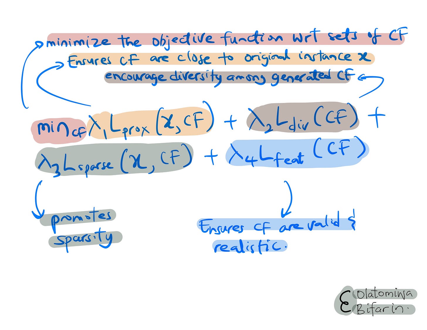
Uses an optimization algorithm to search for counterfactual instances that are close to the original instance but lead to a different prediction. It also promotes diversity by ensuring that the generated counterfactuals are dissimilar from each other.
DiCE selects a subset of the generated counterfactuals that are most relevant and informative to the user. These counterfactuals are then presented as explanations, highlighting the key features that influence the model's prediction.
DiCE uses a distance metric (e.g., Euclidean distance, Manhattan distance) to measure the proximity between the original instance and the counterfactual instances. There is also the diversity metric (e.g., determinantal point processes) to ensure that the generated counterfactuals are diverse. Also, an optimization algorithm is used to search for counterfactual instances that satisfy the distance and diversity constraints.
In brief, we have the following core optimization problem (CF is the set of counterfactual examples and λ are weighting parameters):
As a motivating example, let's take the breast cancer dataset in scikit-learn. The dataset is derived from real-world medical data, containing information extracted from images of breast mass tissue obtained through fine needle aspiration. The dataset comprises 569 samples, each characterized by 30 features that describe various properties of cell nuclei visible in these images. These features include measurements like radius, texture, perimeter, area, and smoothness, providing a detailed quantitative description of the cells' characteristics. The key aspect of this dataset, and while I want us to use it, is its binary classification nature – each sample is labeled as either malignant (cancerous) or benign (non-cancerous).
The code below trains a Random Forest classifier on the dataset and then uses the DiCE (via dice-ml library) to generate and visualize counterfactual examples that would lead to a different prediction for a specific instance (see supplementary code for more information).
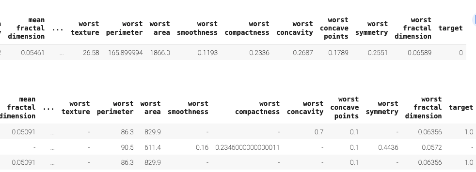
Figure shows a section of the table showing a sample and 3 counterfactuals.
Three CFs are presented with proposed changes in such features as worst perimeter, worst area, worst concave points, etc to flip the class from 0 (benign tumor) to 1 (malignant tumor).
3. Gamma FACET
FACET, a XAI library created by BCG Gamma, is designed to explain global model explanations for ML models. FACET builds directly on SHAP (SHapley Additive exPlanations), by looking at how features interact with each other, specifically in terms of synergy and redundancy.
See my previous article on SHAP:
Synergy is when two features work together to produce an effect that is greater than the sum of their individual effects. For example, consider a model that predicts house prices. While the numbers of beds and baths are individually important, their combination might create a synergistic effect. A house with many bedrooms but few bathrooms might be less desirable than a house with a balanced ratio of bedrooms to bathrooms.
Redundancy is when two features capture the same information. For example, in general, larger houses tend to have more bedrooms. These features are likely to be somewhat redundant, as they both capture aspects of the size of the house.
FACET can be used to identify both synergy and redundancy between features. This information can then be used to improve the model by removing redundant features or by developing new features (feature engineering) that capture the synergistic effects of existing features.
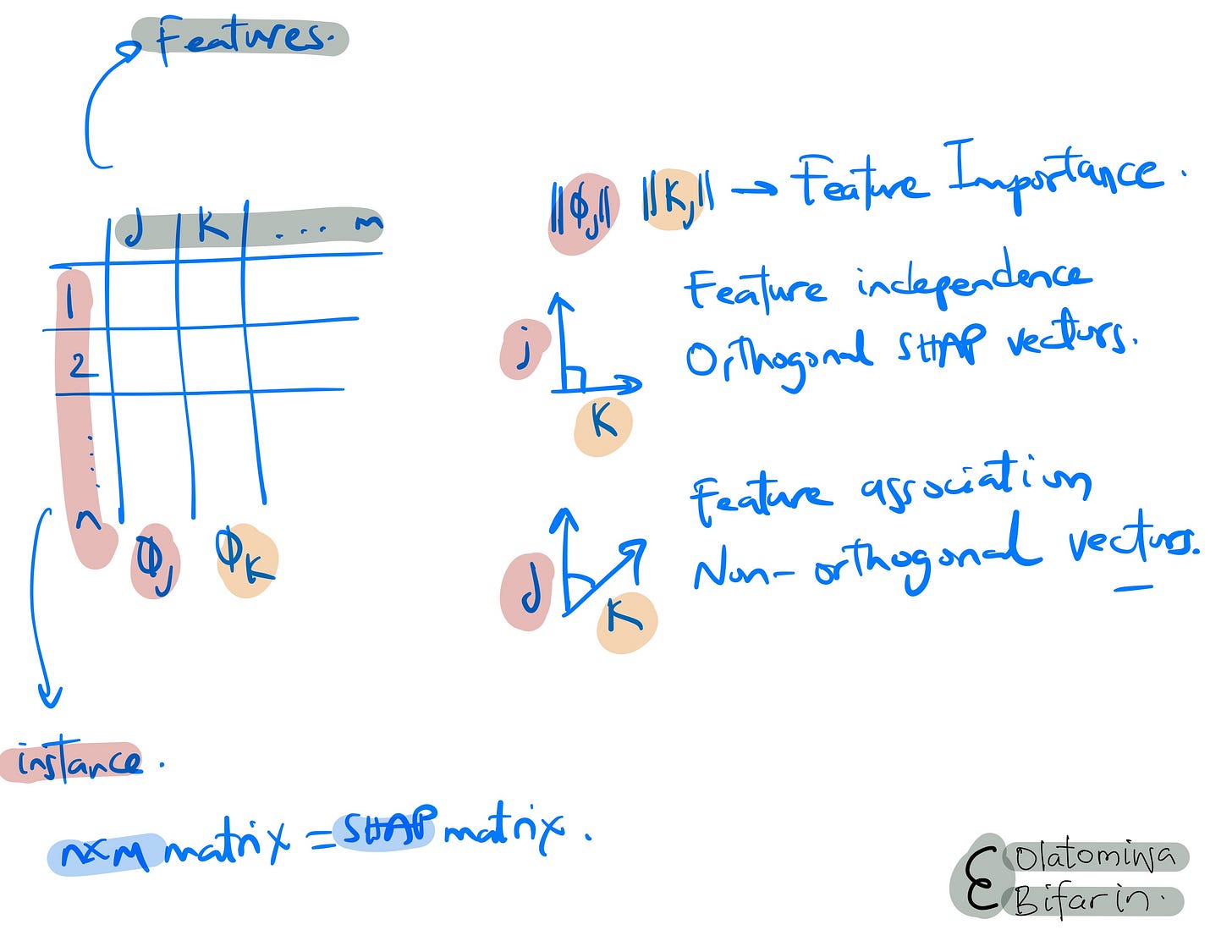
In brief, I think this is how FACET works: it utilizes SHAP values as the basis for its analysis. It then constructs SHAP vectors for each feature, drawing from their SHAP values across different observations. These SHAP vectors are subsequently decomposed into two types of components: orthogonal components, which represent the independent contributions of each feature, and non-orthogonal components, which capture the interactions between features, be it synergy or redundancy. Finally, FACET quantifies feature importance, independence, and the nature of feature associations by examining the magnitudes and angles of these components.
Next, we will use a California housing dataset, which is a built-in dataset in scikit-learn. This dataset contains information about housing in California and it includes features such as: median income in the block, house age, average number of rooms, average number of bedrooms, population in the block, average occupancy etc. The target variable is the median house value for California districts.
In the code below I select the first 500 samples, and prepare it for analysis using FACET. A Random Forest regressor is then created and trained on the dataset. The core of the analysis comes from the LearnerInspector, which examines the trained model's behavior. Finally, the code visualizes two key aspects of the model: feature synergies and redundancies. These visualizations help in understanding how different housing features interact and influence each other in predicting house prices, as well as identifying potentially redundant features in the dataset.
Feature Importance
This is in fact the SHAP values for the features. Median Income (MedInc) is the most important feature that predicts the value of a house, while the HouseAge is the least important of all the features used.
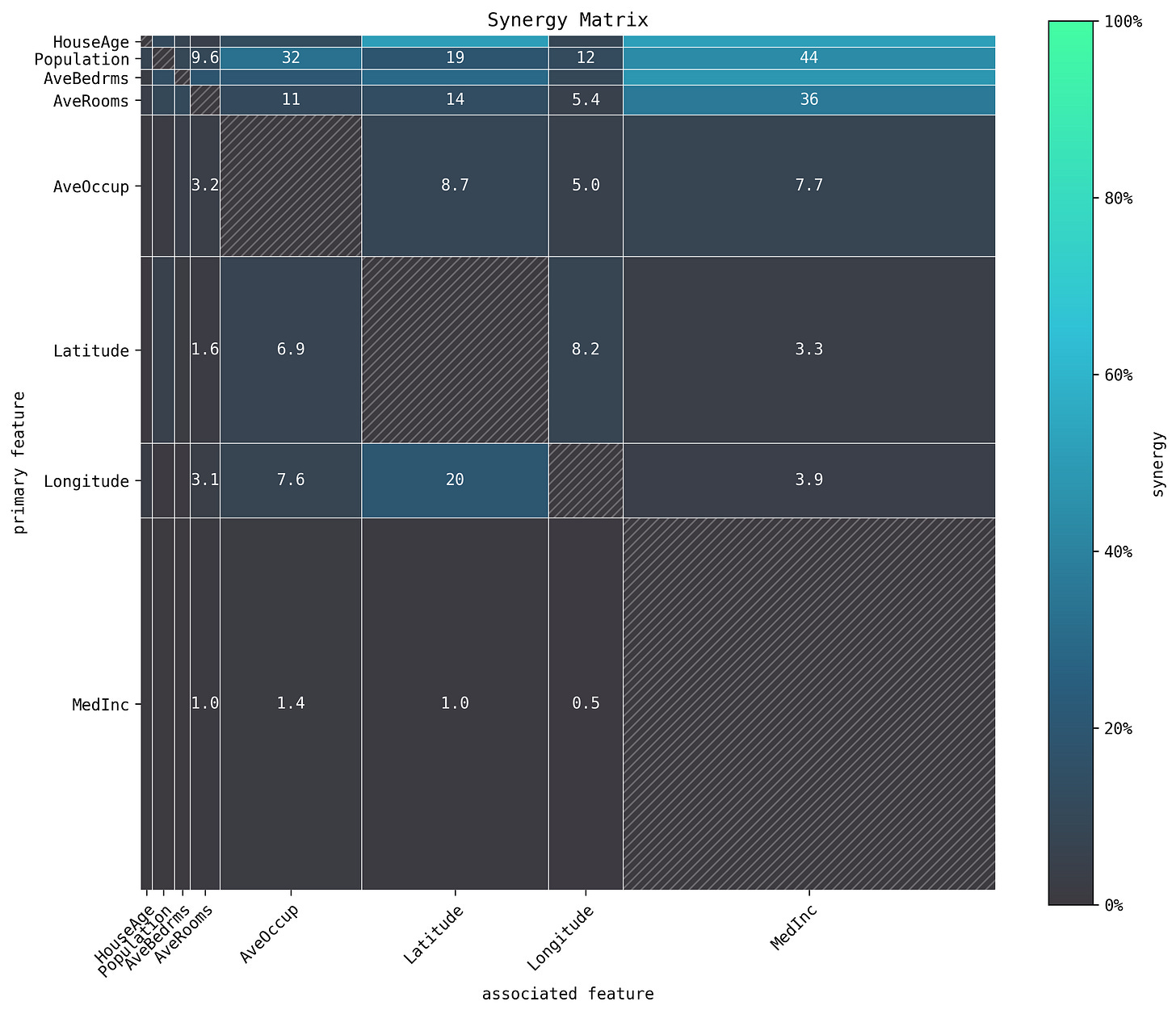
Synergy Matrix
The Synergy Matrix illustrates how features interact to predict the target variable. High synergy values indicate features that work well together in predicting house prices. The strongest synergy is observed between Population and MedInc (44%), suggesting these features combined are particularly powerful in predicting house prices. There's also notable synergy between Longitude and Latitude (20%), which makes sense given their geographical relationship. AveRooms shows good synergy with MedInc (36%), indicating that the number of rooms and income level together are strong predictors.
Also note that the size of each box in the matrix indicates the feature importance.
Redundancy Matrix
The redundancy matrix shows generally low redundancy among features. The highest redundancy observed is between Average number of rooms (AveRooms) and MedInc at 22%. Next to Latitude and Longitude at 19% (not surprising we have some redundancy here given their geographical nature)
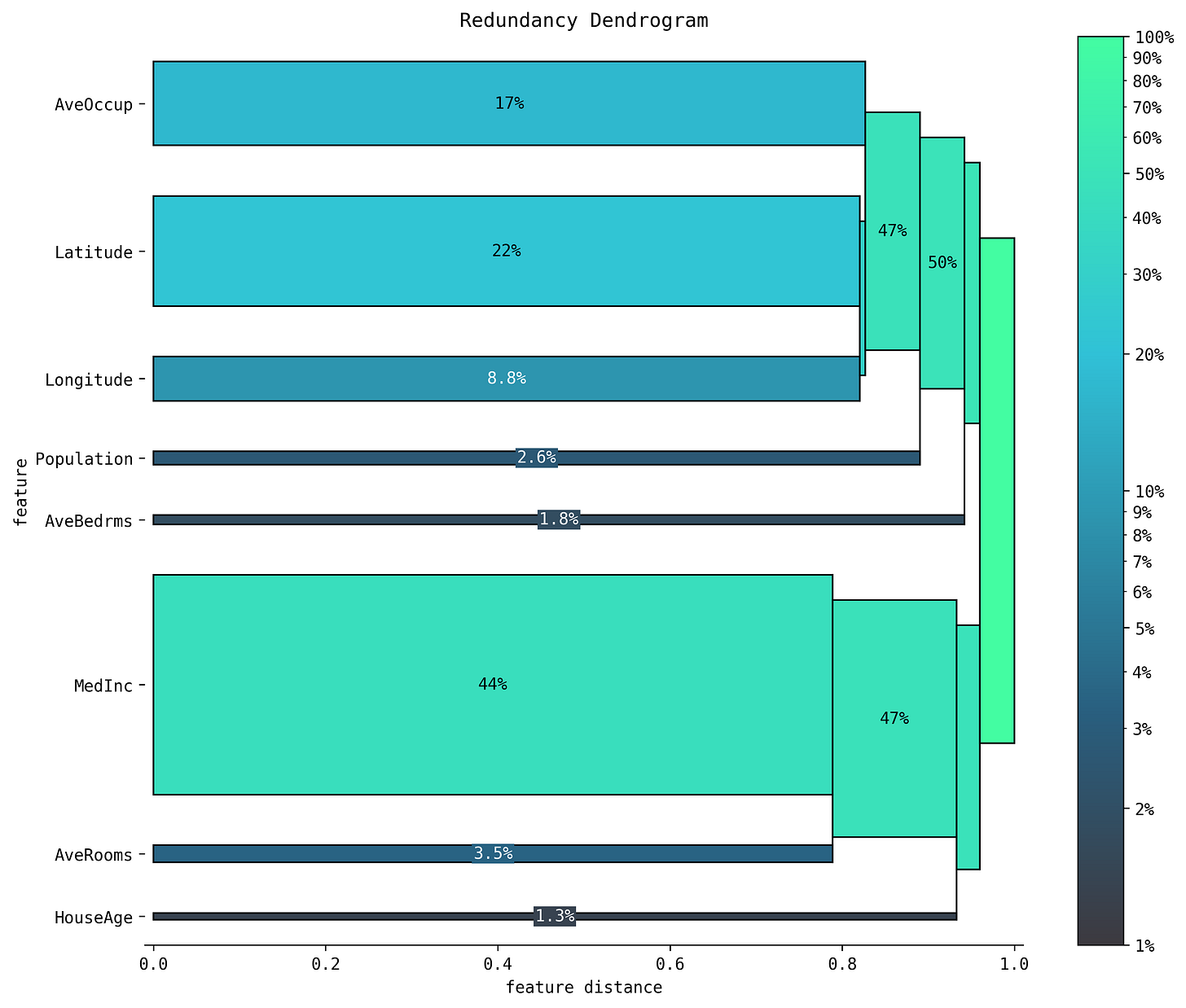
Redundancy Dendrogram
The Redundancy Dendrogram shows the hierarchical clustering of features based on their redundancy - essentially the redundancy matrix presented as a dendrogram. The percentage here represents the feature importance, and how early the features join in the dendrogram represent the redundancy e.g. MedInc and AveRooms join early.
***
In summary, these techniques presented enhance our understanding of ML models, making them more interpretable. By incorporating such methods, we can develop ML models that not only predict accurately but also provide valuable insights into the underlying relationships in the data, crucial for many domains out there, where understanding the 'why' behind predictions is as important as the predictions themselves.
4. References
DiCE GitHub Repo: https://github.com/interpretml/DiCE?tab=readme-ov-file
Ramaravind K. Mothilal, Amit Sharma, and Chenhao Tan (2020). Explaining machine learning classifiers through diverse counterfactual explanations. Proceedings of the 2020 Conference on Fairness, Accountability, and Transparency.
GAMMA FACET: A New Approach for Universal Explanations of Machine Learning Models: https://medium.com/bcggamma/gamma-facet-a-new-approach-for-universal-explanations-of-machine-learning-models-b566877e7812
BCG-X-Official/facet: Human-explainable AI: https://github.com/BCG-X-Official/facet
Jan Ittner & Mateusz Sokół - Exploring Feature Redundancy and Synergy with FACET 2.0: Video Tutorial.


