

Previously: Self Attention
I. Last Time
In my previous blog in this series, we looked at "The Problem with Language," which is the variable nature of input lengths and the inherent dependency of words on other words in a sentence for their meaning. We also discussed how the attention mechanism helps solve these problems, facilitated by such things as the query, key, and value weights, and their mathematical transformations.
In this blog, we will be looking into the complete Transformer architecture.
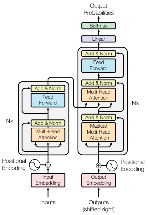
Here is the figure of the originally proposed Transformer model in the Attention is All You Need paper from Google. By the end of this blog my goal is that you have a good idea of what is going on in this figure.
II. Transformer Block
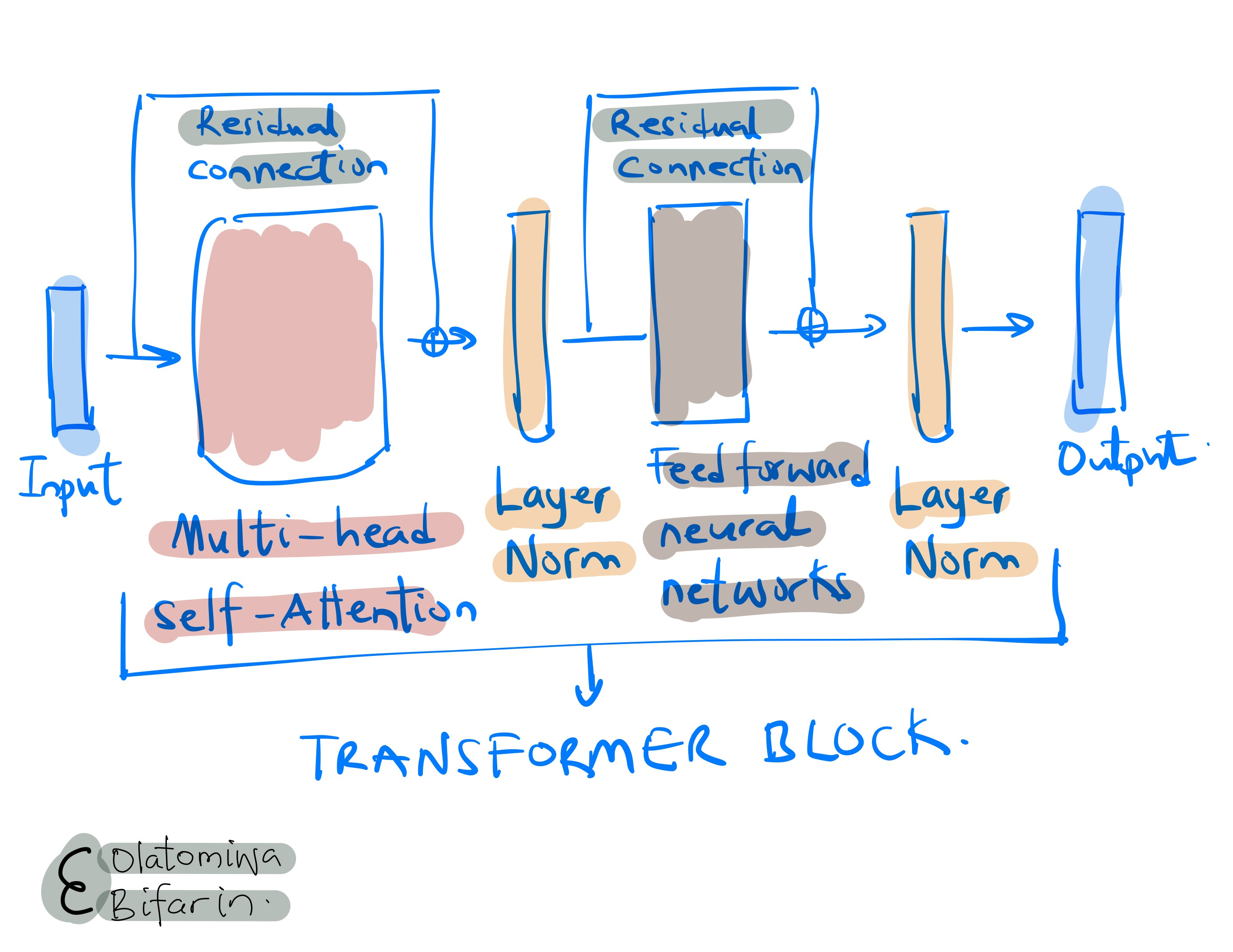
As shown above, the transformer block takes in an input, say a D X N matrix, where the D is the dimension of the embedding vector and N is the number of inputs ( e.g. number of tokens.)

And a series of operation ensues, first we have the multi-head attention block that allows for the interaction of the word embeddings (duly covered in a previous blog). This is followed by a fully connected feed forward neural network.
Furthermore, the self-attention block and the fully connected neural network are followed by a skip connection (residual connection) and a layer normalization operation.
Why layer normalization, why skip connections?
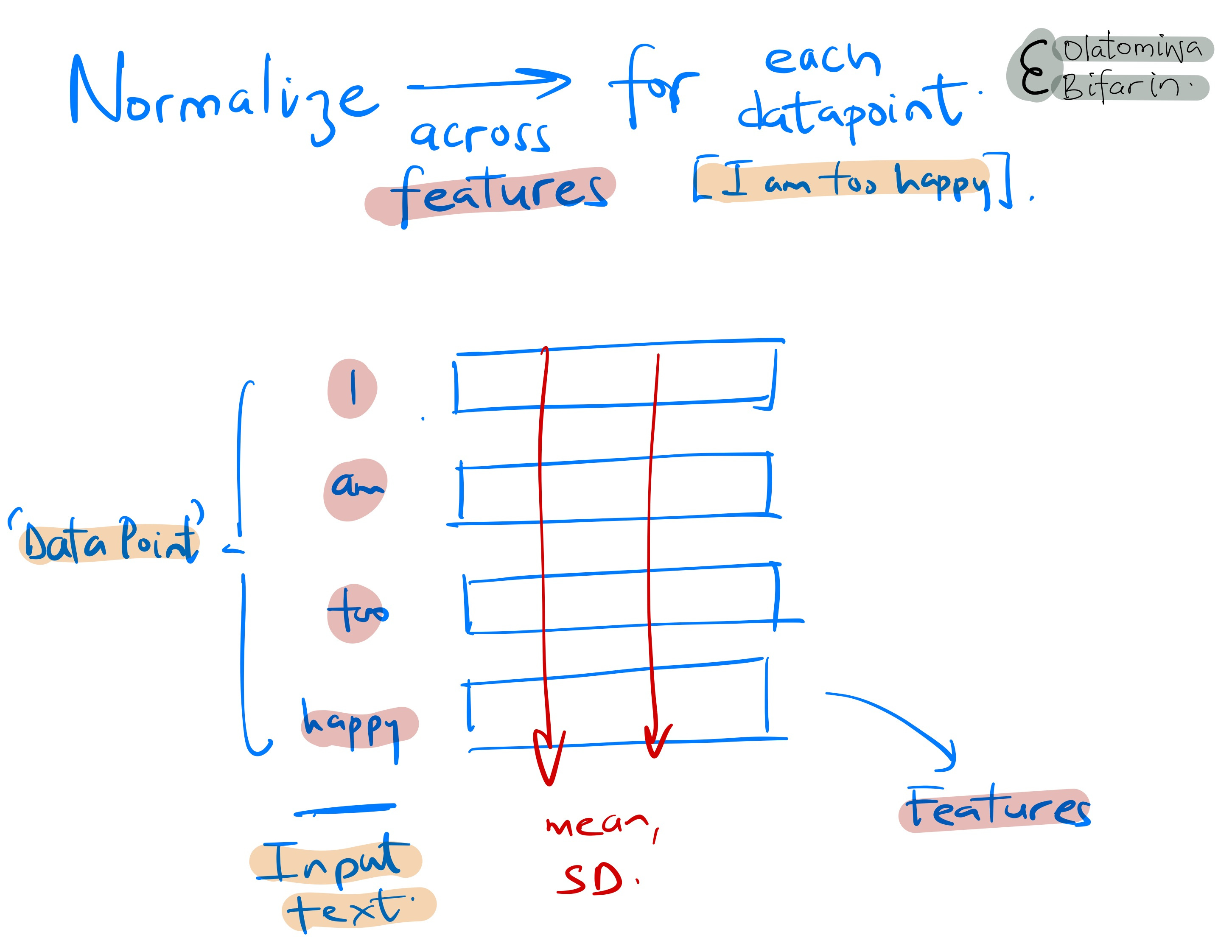
Layer normalization is added to stabilize the learning process by normalizing the activations across the features for each data point.
(A data point is a single instance from the dataset, in the case of text this could be one sentence or one document, on the other hand, sticking to our text example, a feature is the embedding vector for a token, say)
Layer normalization ensures that the scale of the activations (outputs) doesn't become too large or too small, thus avoiding the issues of vanishing or exploding gradients and helping the model to train faster and more effectively.
Residual connections, on the other hand, are introduced to allow gradients to flow directly through the network, mitigating the risk of gradient vanishing during backpropagation in deep networks.
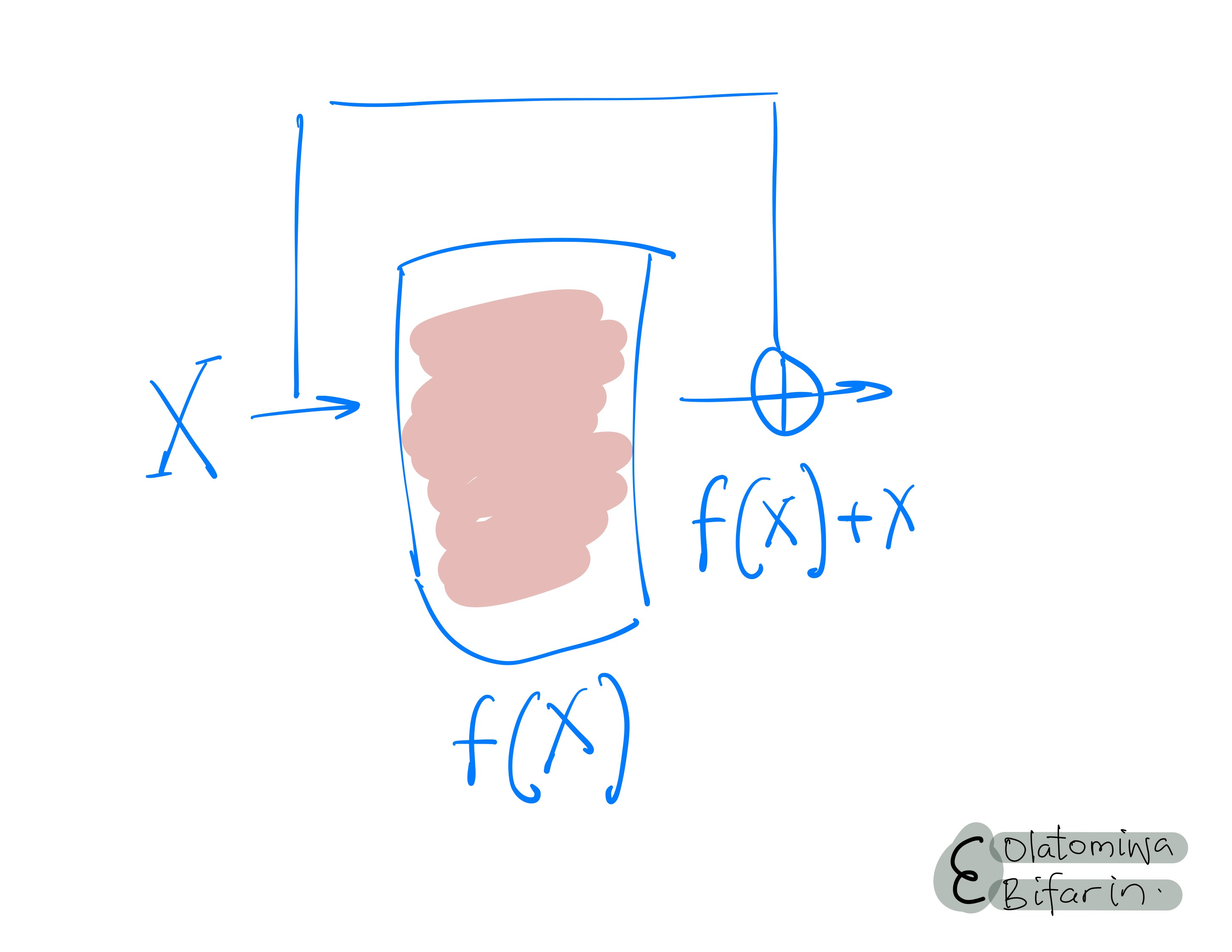
They enable the training of much deeper models by allowing the information to bypass parts of the network, leading to improved learning efficiency and easier optimization.
In the case of fully connected feed-forward network, it is essential for providing the model with the capability to learn complex patterns, introduce non-linearity (through its activation functions such as ReLU), increase model capacity (i.e., the number of learnable parameters), and maintain position-wise processing for handling sequences.
Now that we know what a transformer block looks like and how it works, there are different ways they can be put to use.
In brief, we have the encoder-only models, the decoder-only models, and the encoder-decoder models. We will go through them in turns.
III. Encoder Models
This model transforms the inputs in such a way that it can support a wide variety of downstream tasks like dimensionality reduction, named entity recognition, etc. A popular example of the encoder model is BERT (Bi-directional Encoding Representations from Transformers).
They come in two primary sizes: BERT-Base and BERT-Large. Let’s open up BERT-Large and let see what is inside.
The dimension of word embeddings is 1024. Furthermore, the number of transformer blocks is 24, while the number of self-attention heads in each block is 16. With a word embedding size of 1024 and 16 attention heads, the size of the query, key, and value matrices for each head would be 64 (1024/16).
The dimension of the single hidden layer in the fully connected feed-forward network within each transformer block is also 4 times the size of the word embedding dimension, so we have 4096 (4 X 1024).
And finally, the total number of parameters in the model is 340 million (You might think that is large already, but let’s get to the GPT series).
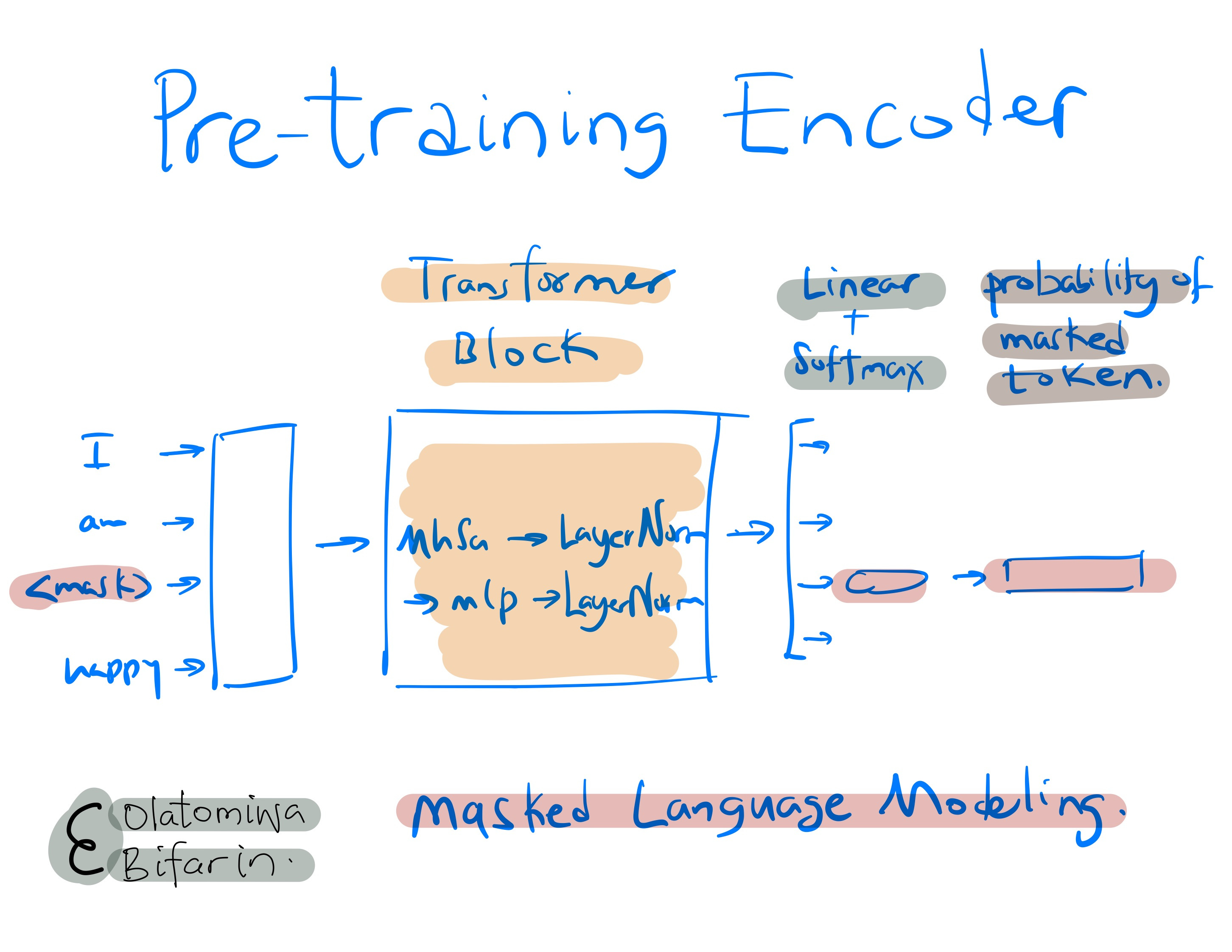
Talking about training task, it entails pretraining and finetuning. Pre-training involves self-supervision where, for example, Masked Language Modeling (MLM) can be used (The approach involves concealing certain words within the input text at random and instructing the model to deduce the concealed word, relying on the surrounding context for clues. This method teaches the model on the significance of individual words and their contextual relationships.)
Another example is Next Sentence Prediction (NSP), which considers the sequence of sentences as an implicit "label," training the model to determine whether two sentences follow each other sequentially.
In finetuning, the goal is to adapt pre-trained model to a specific downstream task such as question answering, sentiment analysis, or text summarization.
I will give a domain specific example, and then we will look at the architecture of the famous of them all, GPTs.
PubMedBERT: a model I am currently utilizing for my research to follow-up with trends within a field in the biomedical space. PubMedBERT adopts a self-supervised learning method specifically designed for biomedical research papers. It was trained from scratch leveraging an extensive 21GB dataset from PubMed, a rich source of biomedical literature.
This model diverges from conventional tasks, focusing instead on domain-specific challenges such as predicting masked biomedical entities and analyzing sentence pairs to comprehend the dynamics of, say protein interactions.
Through self-supervised training on these unique tasks, PubMedBERT is primed for a range of biomedical NLP applications, including entity recognition and so on.
IV. Decoder Model
The architectures of the encoder and decoder model are very, very similar, nevertheless, the objectives vary significantly. The encoder is designed to create a comprehensive representation of the text, which can then be adapted to address a broad spectrum of specialized NLP tasks.
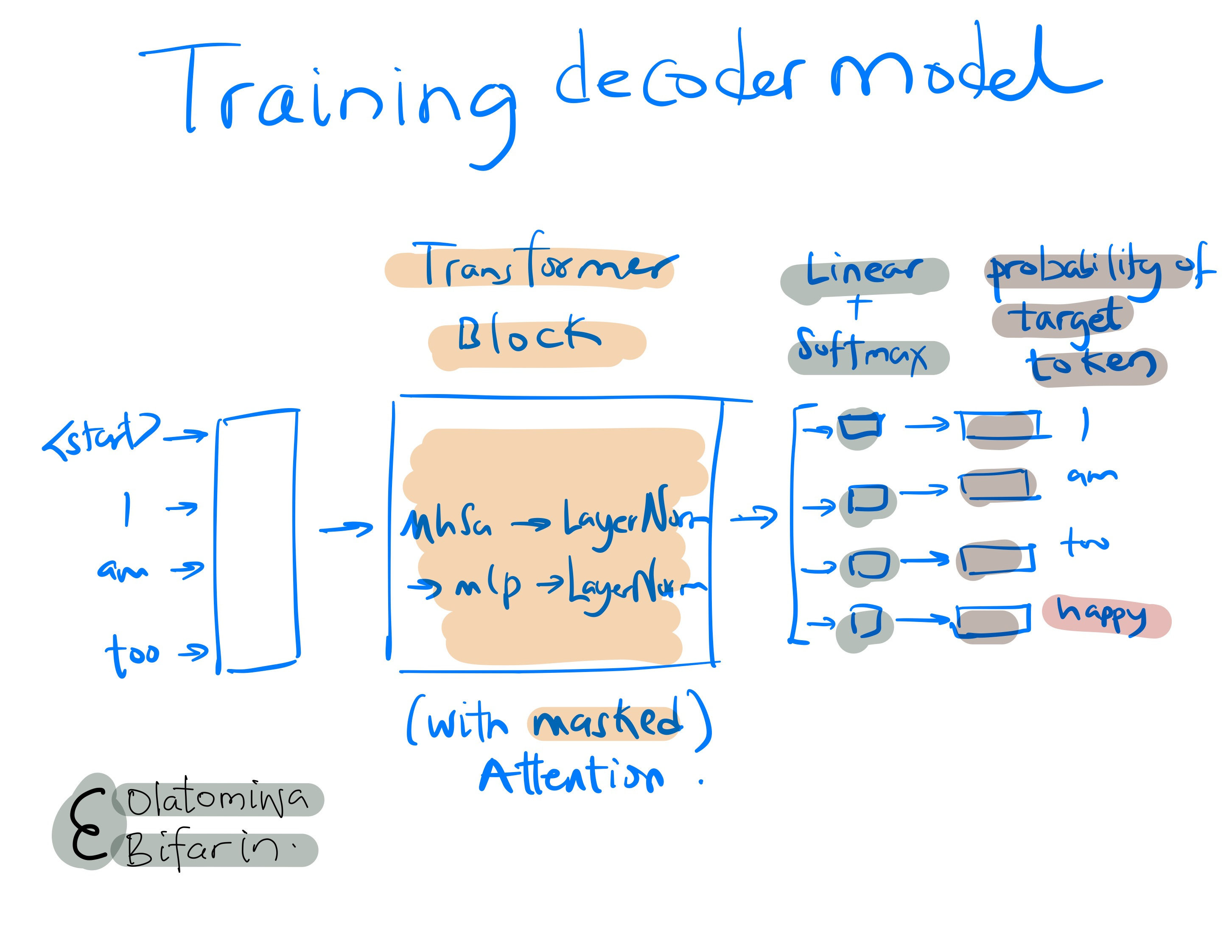
On the other hand, the decoder model is strictly focused on the generation of the next token within a sequence. The GPT (Generative Pre-trained Transformer) series of model is an example of a decoder only model. In this session, we will home in on GPT-3.
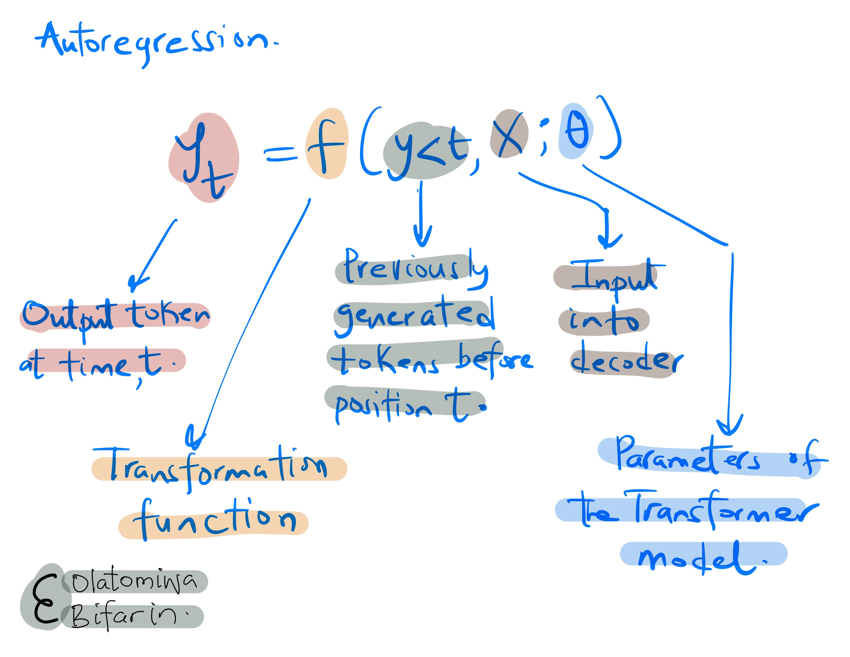
GPT-3 utilizes an autoregressive language model. This method focuses on refining the likelihood of what comes next based on the existing context, thereby allowing the model to form a detailed statistical map of the text.
Another important concept is the masked self-attention. GPT-3 employs masked self-attention mechanism, an approach that guarantees that when the model calculates self-attention, each token is only influenced by itself and the tokens that appear before it in the sequence, excluding any subsequent tokens. This feature is vital for preserving the model's autoregressive characteristic, ensuring that the prediction of each word relies entirely on the preceding words.
When chatGPT was released, many people were rightfully wondering what sort of miracle was going on behind the scenes. If you have read this article up to this point, you should be well aware that such miracles are just mathematical computations.
Now let’s put the final nail on the coffin: Token by Token Generation.
Since the autoregressive language model establishes a probabilistic framework for sequences of text; it enables the generation of new, plausible text samples. So next time you see the text streams pile up on your ChatGPT app, you know what’s going on.
Other decoder model powered-products you might be familiar with include Bard (now Gemini), Claude, and LLaMA.
Beginning with an initial input, say a prompt from the user, GPT constructs text one token at a time. At every step, it employs its previously learned parameters along with the context from earlier tokens to predict the upcoming token.
And I should say that the best performing models are built by manipulating an ungodly amount of numbers (we will talk a bit more about this in our final section – variables in Transformers).
In the meantime, let us treat the third type of architecture – the Encoder-decoder model.
V. Encoder-decoder Model
In the encoder model, we don’t get any generation of new tokens, whereas, as we have seen, in the decoder only model, we do.
On the other hand, what we have with the encoder-decoder model is an input sequence coming in and an output sequence going out. In other words, what we are talking about here is a sequence-to-sequence task.
Say you have a set of English poems, and you want to translate it to Polish really bad, an encoder-decoder model can perform such machine translation task.
To do this, we will need a variant of the self-attention mechanism, called cross attention.
Here is how it works (i.e., how we train the model): the English sequence will be the input for the encoder part of the model. It does its thing with the self-attention and what-not.
Next, the output of the encoder part of the model (which is an enriched representation of the English sequence), is passed into a transformer block in the decoder part of the model.
This transformer block in the decoder uses the masked self-attention (as previously described). Importantly, the output from the encoder’s transformer block is used for the attention mechanism in the selected transformer block of the decoder.
Hence cross-attention.
During back-propagation, the decoder learns the pattern of matching the output of the encoder, with its own processing.

VI. Variables in Transformers
To sum up this presentation, it will be useful to state (restate) some of the important variables in Transformers. I will divvy them up based on where they come in the training process.
We have the 1) inputs into the model. 2) Internals of the model, and 3) variables associated with the actual training.
Inputs
Vocabulary Size: The total number of unique words or tokens the model can understand and generate.
Embedding Size: The dimensionality of the vector representations for each token in the model's vocabulary.
Sequence (Context) Length: The maximum number of tokens the model can process in a single input sequence.
Internals
Number of Attention Heads: The count of parallel attention mechanisms used to capture different aspects of the input data's relationships.
Intermediate Size: The size of the feed-forward layers within each Transformer block, often larger than the embedding size.
Number of Layers: The number of Transformer blocks (each containing self-attention and feed-forward networks) stacked to form the model.
Training
Batch Size: The number of training examples processed simultaneously during the training phase.
Tokens Trained: The total number of tokens the model was exposed to during its training process.
Number of Parameters: The total count of trainable weights and biases in the model, reflecting its complexity and capacity for learning.
To give you an example of the scale of the computation that could happen with these systems, GPT-3 has 175 billion parameters, while GPT-4 is suspected to have more than a trillion parameters! And for the magic behind the model, we are talking about the astounding number of text (in the case of multi-modal models, also images, video and audio) on the internet.
As I am writing this line, I got a bit distracted by the news of Gemini 1.5 from Google, which they say outperforms GPT-4, we are talking about a context window of up to 1 million tokens here (vs 128,000 tokens in GPT-4)
Brave new world!