

This will be my first blog entry on The Epsilon, and I have pondered so much on how to approach the difficulty level, and the length of my posts. I am still somewhat in the mood of pondering but in the meantime, I have decided to start with beginners friendly blogs, and gradually dial up the difficulty level overtime. For the length, this might be variable, some will be long, some will be supershort. Also, there will be a monthly newsletter that will cover contents on machine learning, data science, AI, and AI X Bio, so don’t forget to subscribe away!
With the housekeeping out of the way, let’s get on with it.
supplementary code for ML primer
I. Definitions
My favorite definition of machine learning is Tom Mitchell's, so we will start with that:
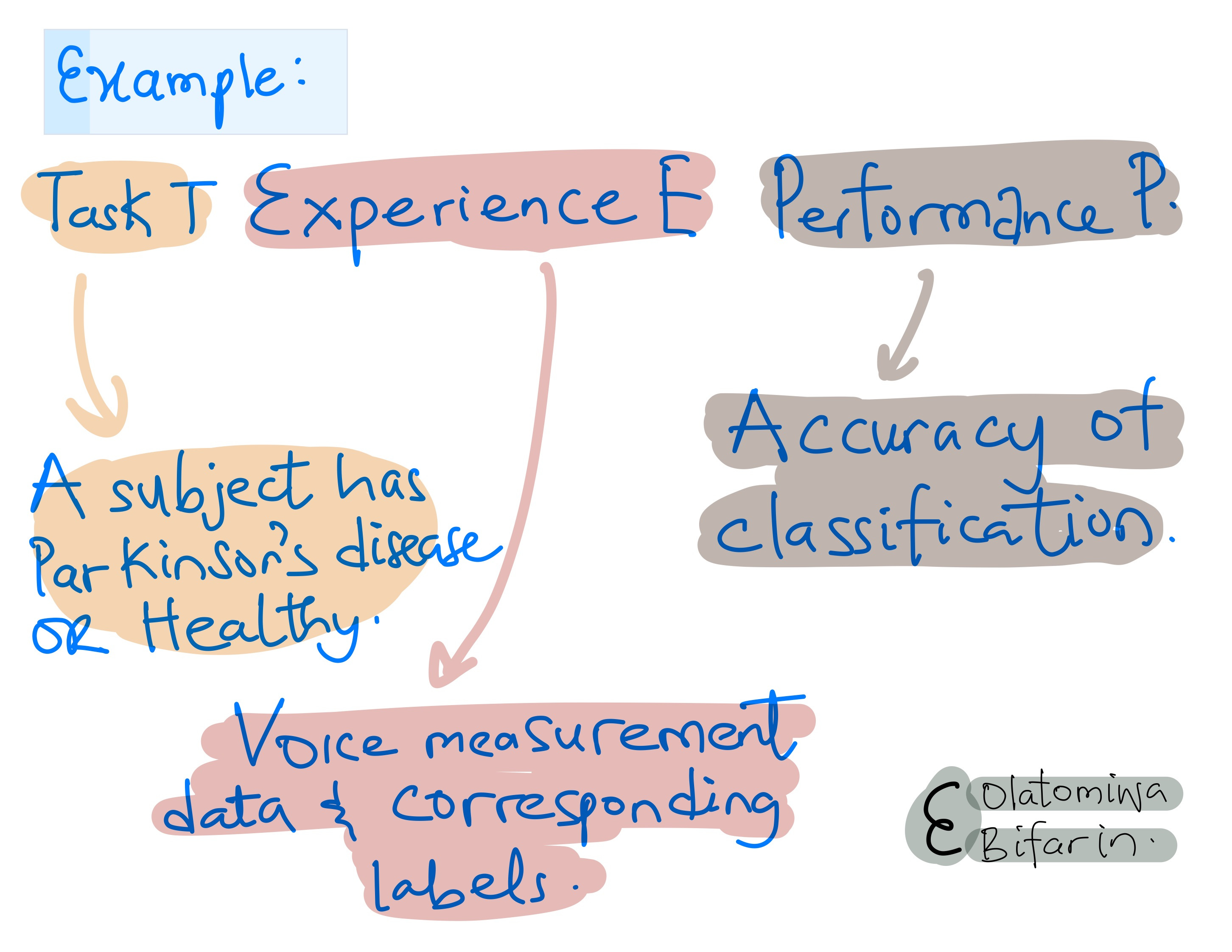
"A computer program is said to learn from experience E with respect to some class of tasks T and performance measure P, if its performance at tasks T, as measured by P, improves with experience E."
The goal is to approximate a function. More formally:
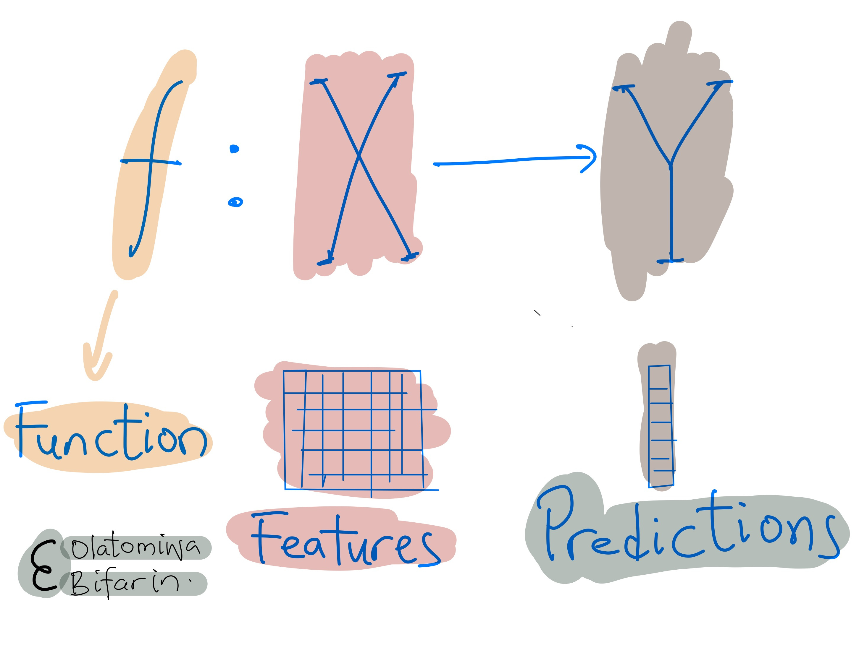
The function (your machine learning model) maps features to classes.
II. ML Tasks
As you might have guessed, there are different types of task T, and the different kinds of task T would be handled differently. Take the Parkinson's disease example above, it is called a classification problem, expressed in its simplest form: binary classification. A or B. Disease or Healthy. Let's say a few things about this (and similar) problems before I proceed to some other machine learning problems.
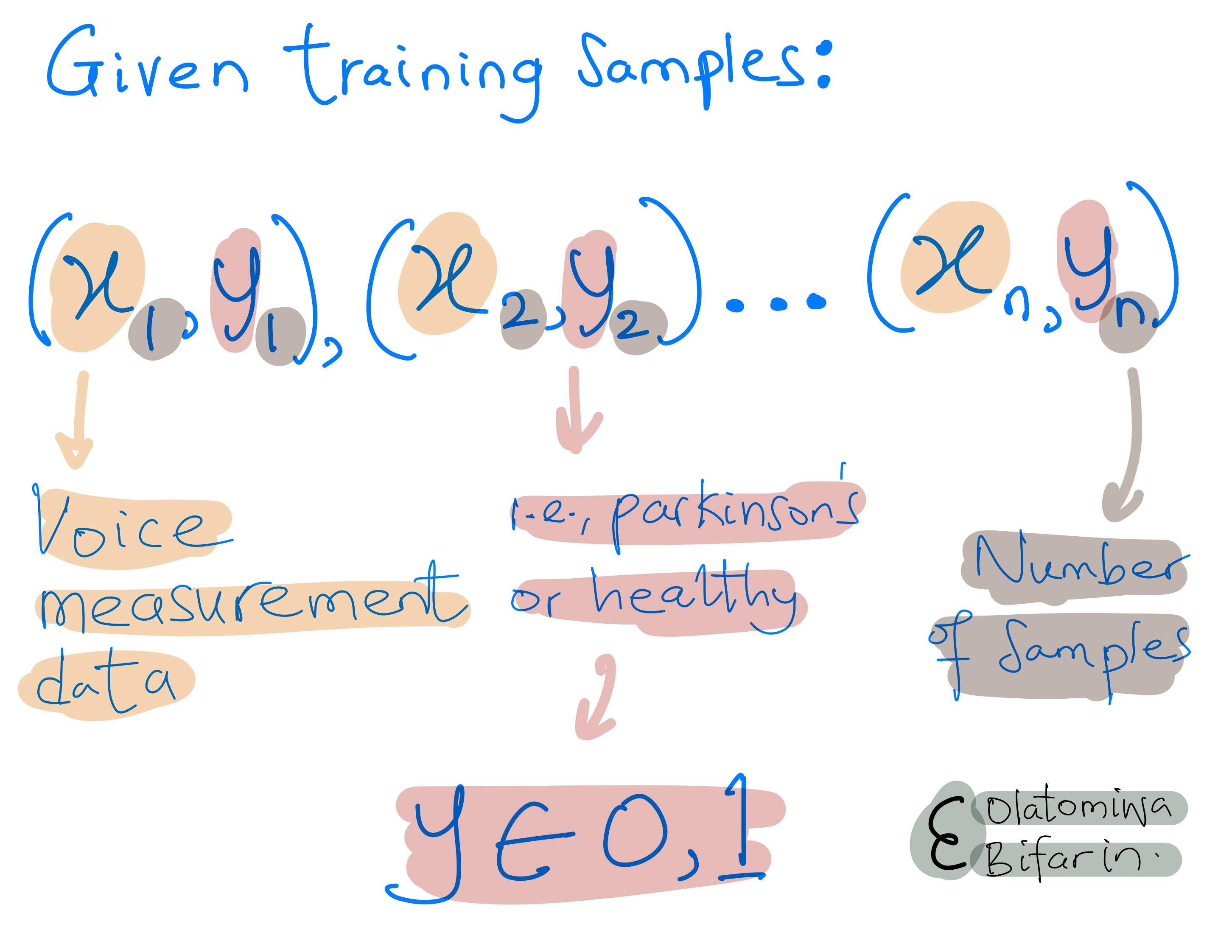
The goal is to train a model and make a prediction on unlabeled voice measurement data. Once a prediction is made, we want to capture if we are doing well. For a binary classification problem, we can approach it this way:
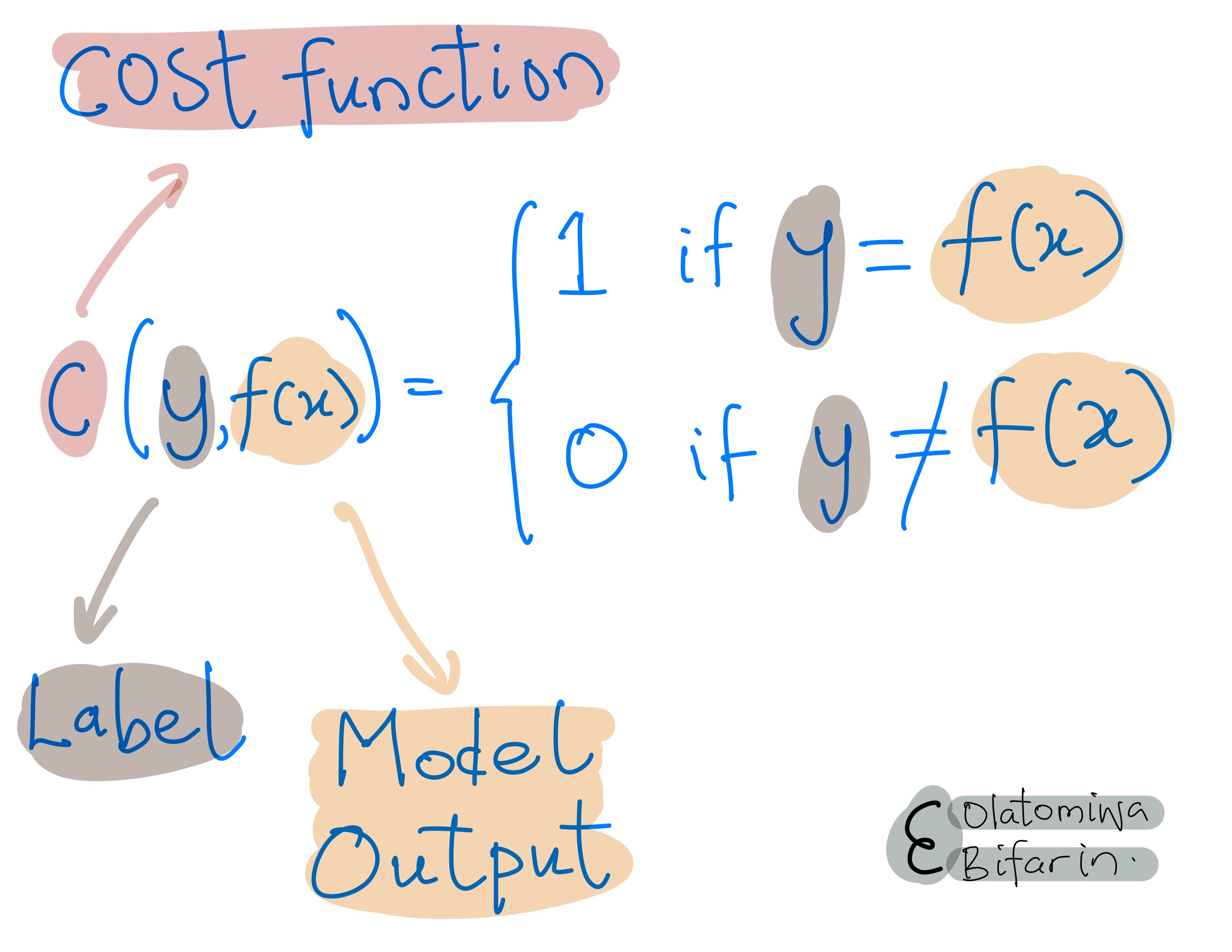
This expression defines a cost function that takes two arguments: label (ground truth) and model output. The function returns 1 if ground truth equals model output and returns 0 if ground truth does not equal model output. We can tabulate our results, and we have the model's accuracy.
We can use other metrics, such as the F1 score and Matthews Correlation Coefficient (MCC), but we have a bigger fish to fry in this blog, so I will skip it.
So far, we have been treating a binary classification task which is a kind of supervised learning – supervised because we have the labels. And it doesn't take much to figure out that the other kind is called unsupervised learning, a machine learning task where there are no labels.
The algorithms that fall under this category are left to find patterns and relationships within the data on their own without any explicit guidance.
And yet, in some other cases, the goal of machine learning is not to predict a qualitative variable but a quantitative variable. For example, in a medical context, one might try to predict the size of a cancerous tumor based on quantified metabolites in a patient's urine (Fun fact, I attempted this in grad school). This type of task is called a regression task.
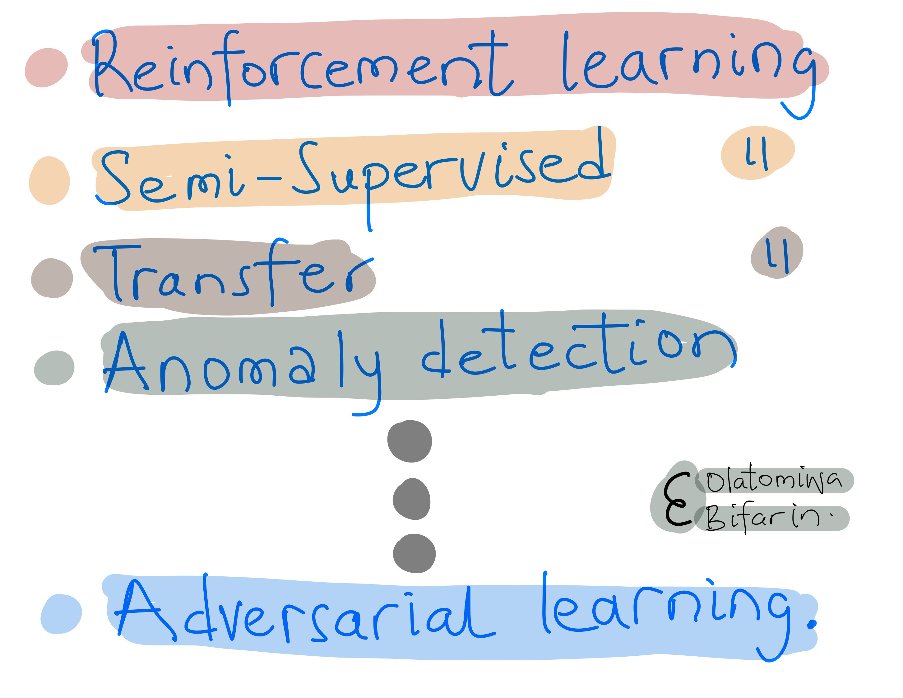
And I would be remiss if I didn’t state that there are many, many, many more machine learning tasks that are beyond the scope of this brief explanation.
III. A Few ML Concepts
IIIa. Model Fitting
Of what use is a car that cannot move? Of what use is a machine learning algorithm that cannot learn (i.e., generalize)? And a ML algorithm generalizes well when it does not underfit or overfit.
This simple analogy will work. Take a 12-year-old girl studying for an exam, one could think of two ways she could fail the exam. 1) If she fails to study the materials well enough, 2) If she memorizes the examples in the class notes and fails to understand the concepts that will be tested in an exam.
1) is the analogy for underfitting: this is the case when the ML model fails to generalize because it hasn't learned the pattern in the training dataset well. For point 2), the analogy works for overfitting: a model overfits when it has memorized the training data so well that generalization on the test data fails.
The graph below will give a little more context.
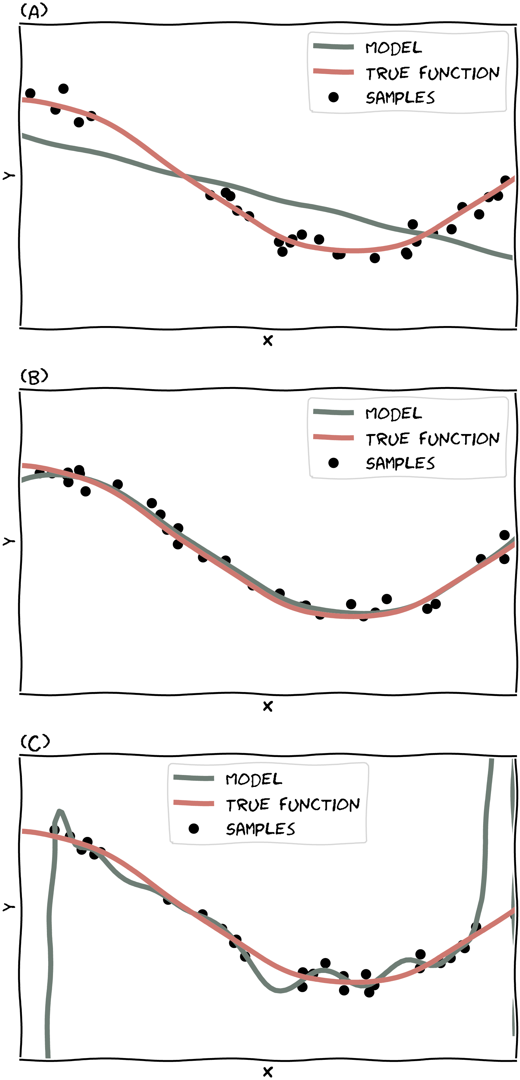
Say the samples plotted are the training data, and the graph shows the true function and the function learned by the model. The linear function (our model) in (A) will likely underfits.
It’s unlikely the model will fit validation data with similar data distribution since it’s just a straight line. (The way we check for under/(over)fitting is to check if the model generalizes from the training data.)
The model in the middle (B) fits the true function pretty well.
For (C), we see a model which gives us an idea of what it means for a model to overfit the training data. The model tries hard to hit on every single data point, and this will only guarantee one thing – poor performance on the validation dataset.
IIIb. Inductive Bias
In philosophy, Inductive reasoning refers to the process of drawing a conclusion based on the premise that does not necessarily guarantee the conclusion. This is distinct from deductive reasoning, where the premise logically entails the conclusion.
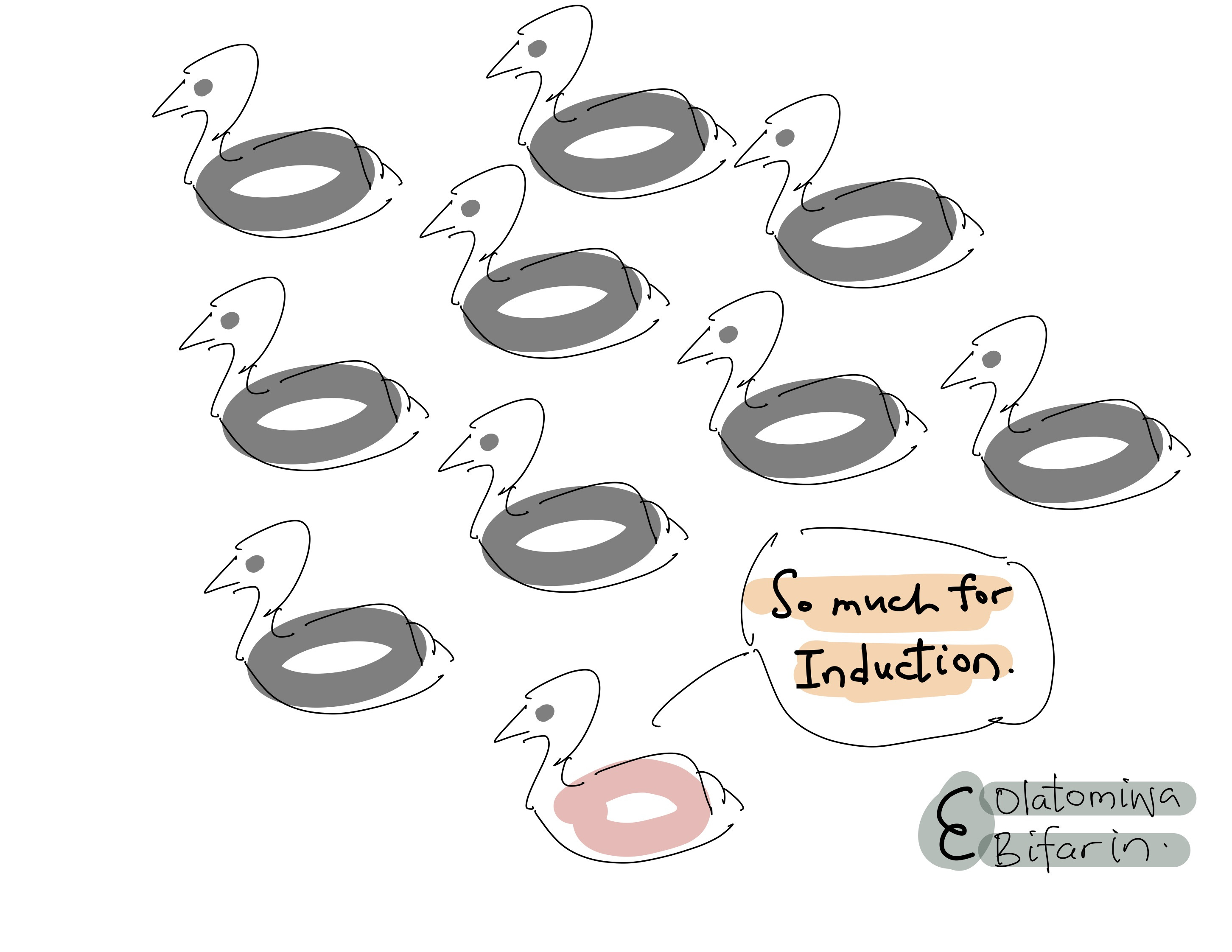
For instance, an example of inductive reasoning is the argument that all swans are black based on the observation that all swans one has seen so far are black.
Premise: Every swan that I have seen is black.
Conclusion: Therefore, all swans are black.
In machine learning, training models with training data and using them to make predictions on test data is a form of inductive reasoning. The different ways in which machine learning algorithms perform this task are known as the induction bias or learning bias, which reflects the assumptions that the algorithms make.
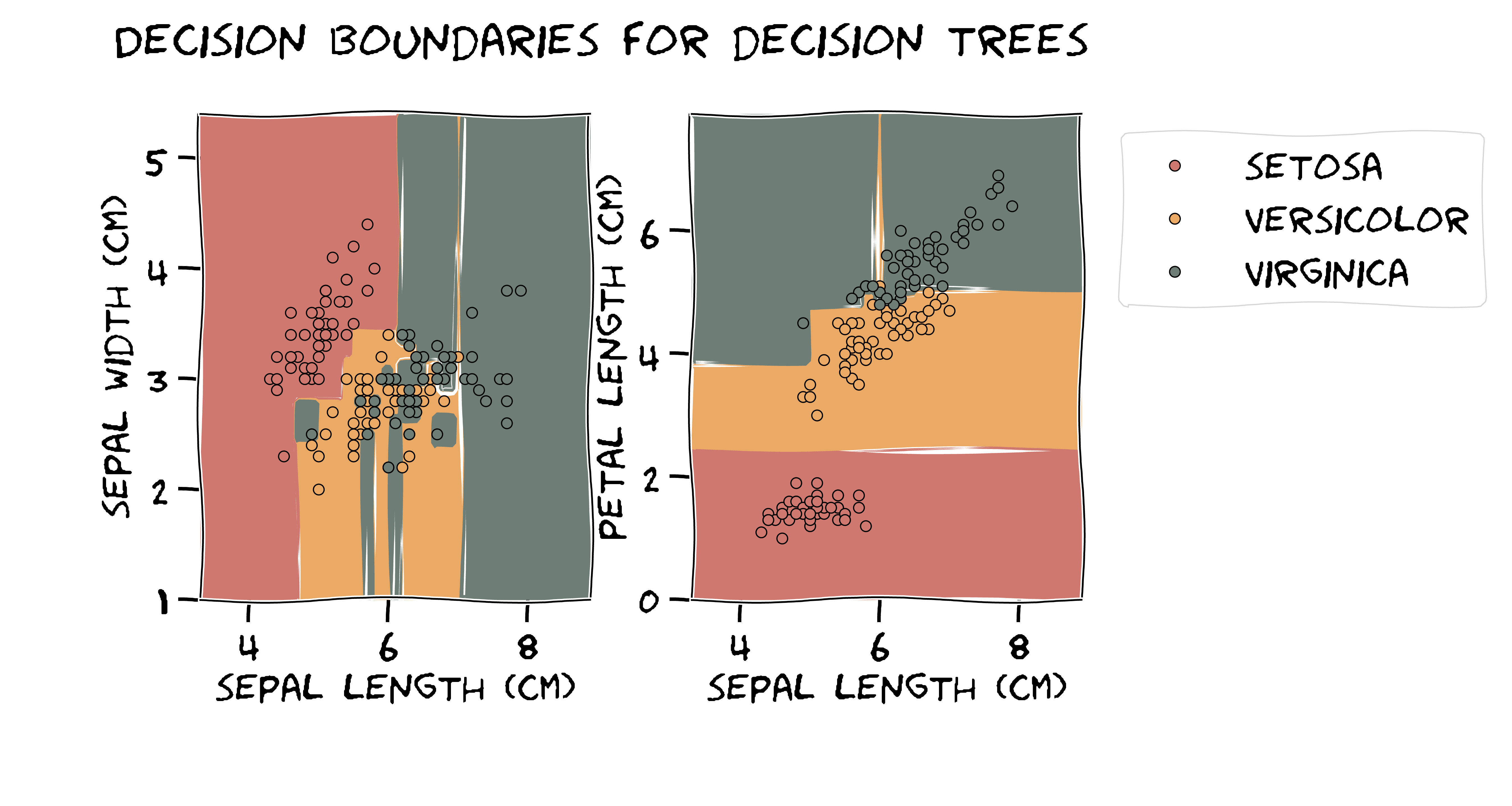
Take decision trees:
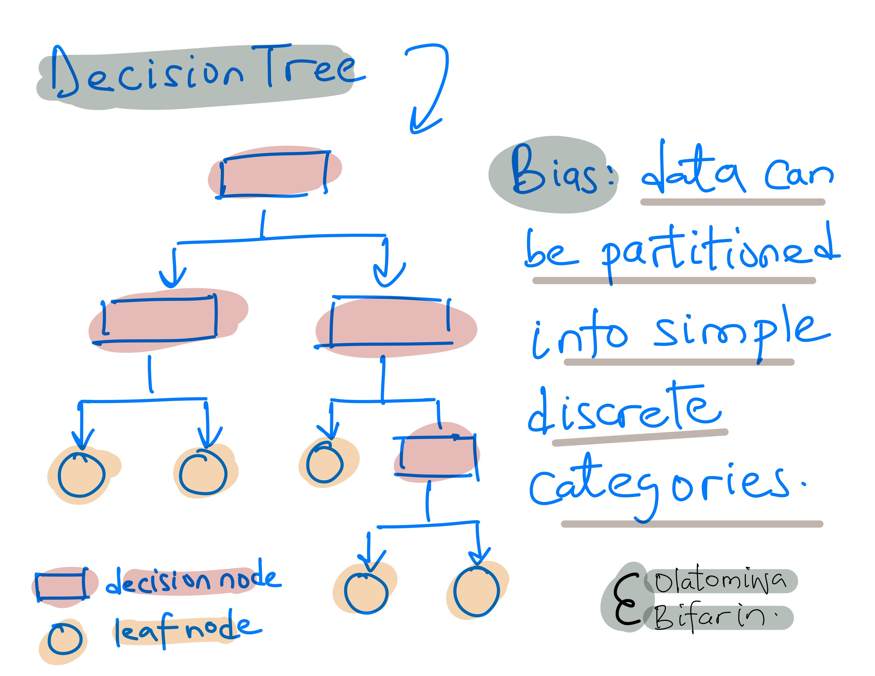
Working with the famous iris dataset, here is what the decision boundaries of a decision tree look like. Piecewise linear, axis-aligned, and hierarchical partitioning of the feature space. All these are because of the inductive bias it adopts.
Friends, contrast decision trees with support vector machines which assume that data are linearly separable and can be divided into different classes based on their distance from a hyperplane.
Or K-Nearest Neighbors: Closer samples (in the Euclidean space, defined by k-NN) are more likely to be the same. Or even linear regression: A linear relationship between the features and the response variable.
And I can go on, but there will be no end to this blog. So, I would stop here. And expect that some of the themes mentioned here might be explored in depth in future blogs.