


In the next couple of blogs - or so; I will be exploring some explainable AI techniques (XAI). I am starting with LIME largely because it will be a nice segue into the more popular technique, Shapley Additive Explanation (SHAP).
Supplementary code for LIME.
The interpretability of machine learning (ML) models has become a crucial aspect in deploying the models. The need for interpretability arises from the fact that many real-world applications, such as medical diagnosis, have high stakes and require a clear understanding of the decision-making process of the model. In this blog, we will be unpacking one such method.
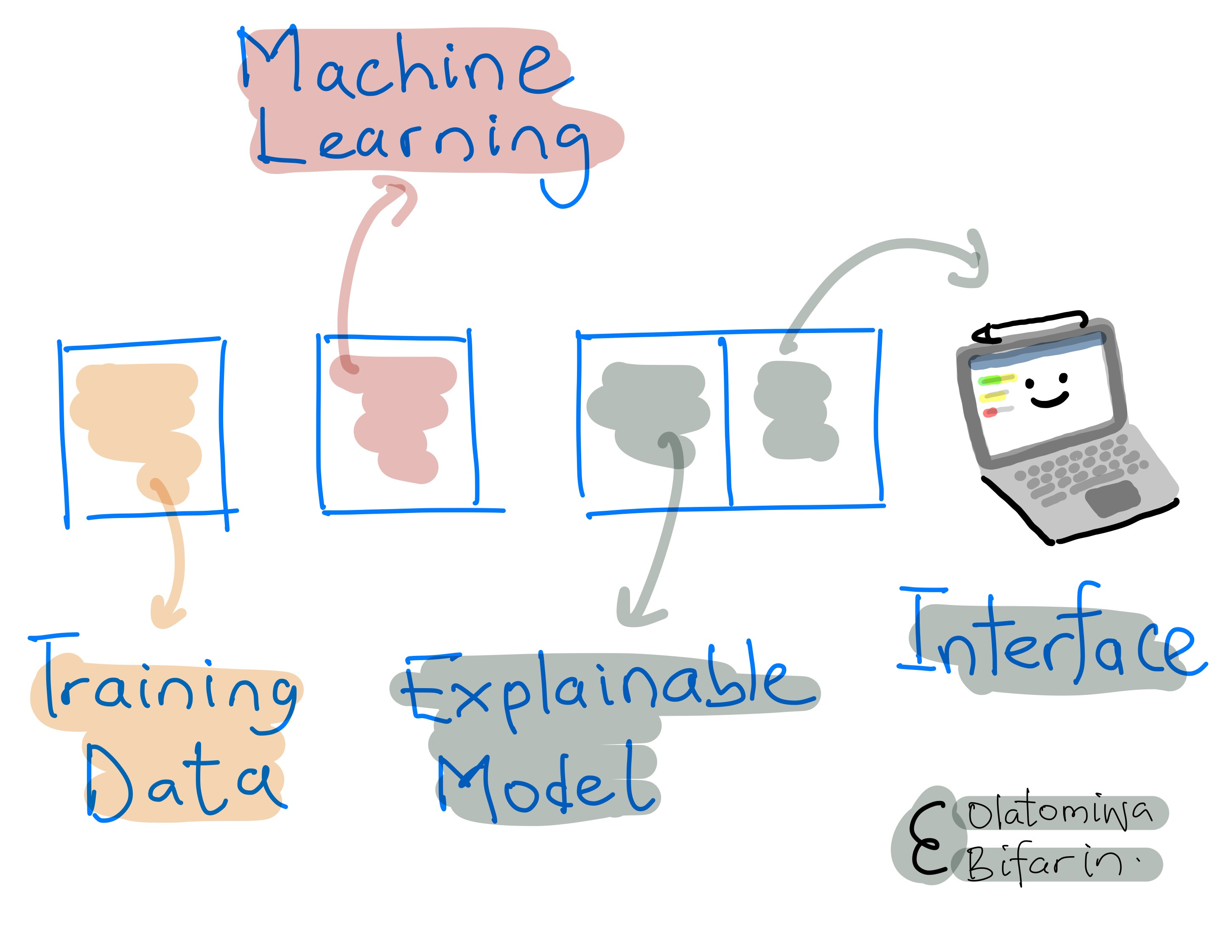
Local interpretable model-agnostic explanation (LIME) is a technique that is used to explain ML model's prediction at a local level. i.e., it explains the prediction of individual instances in your dataset.
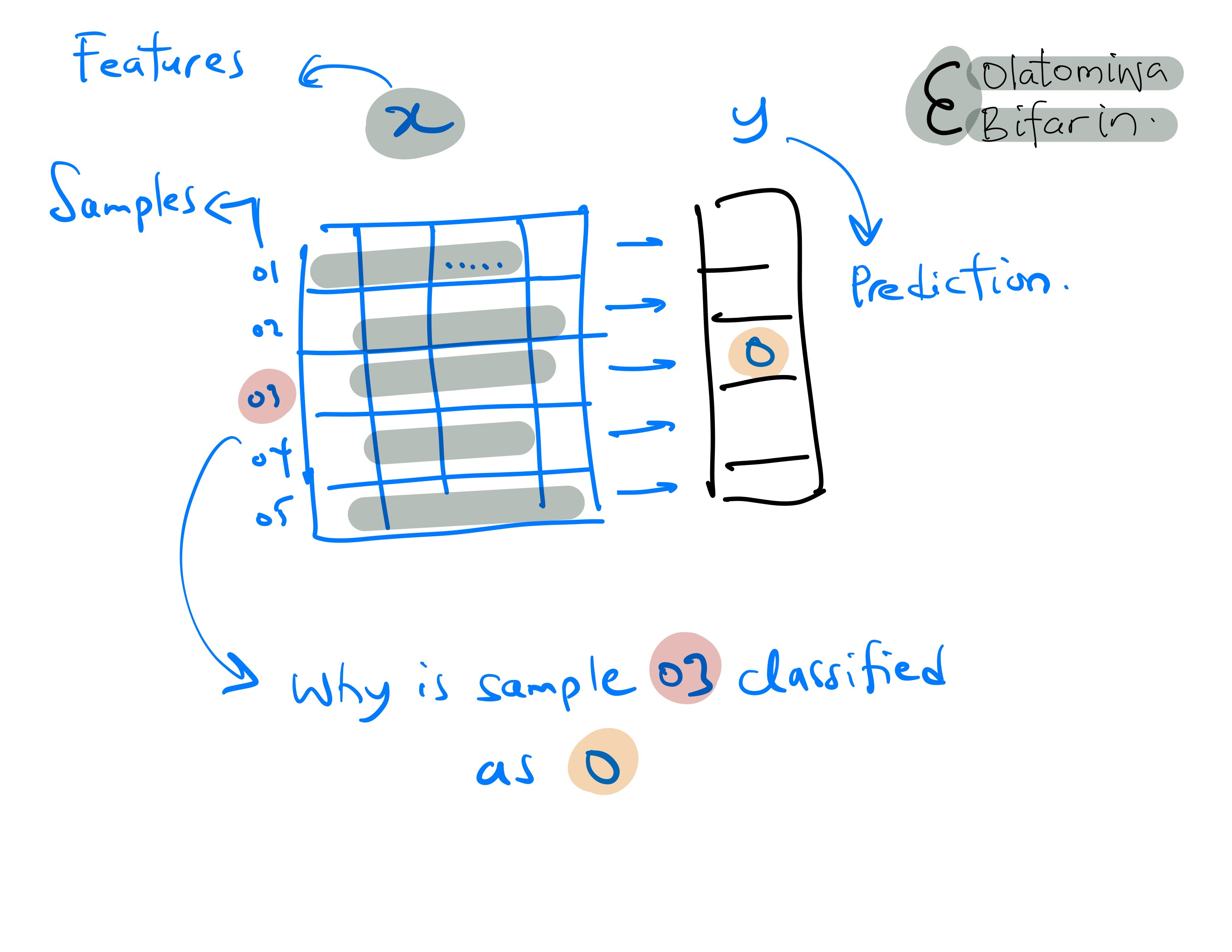
The technique can be used to explain models of any type and are, as such, called model agnostic XAI technique.
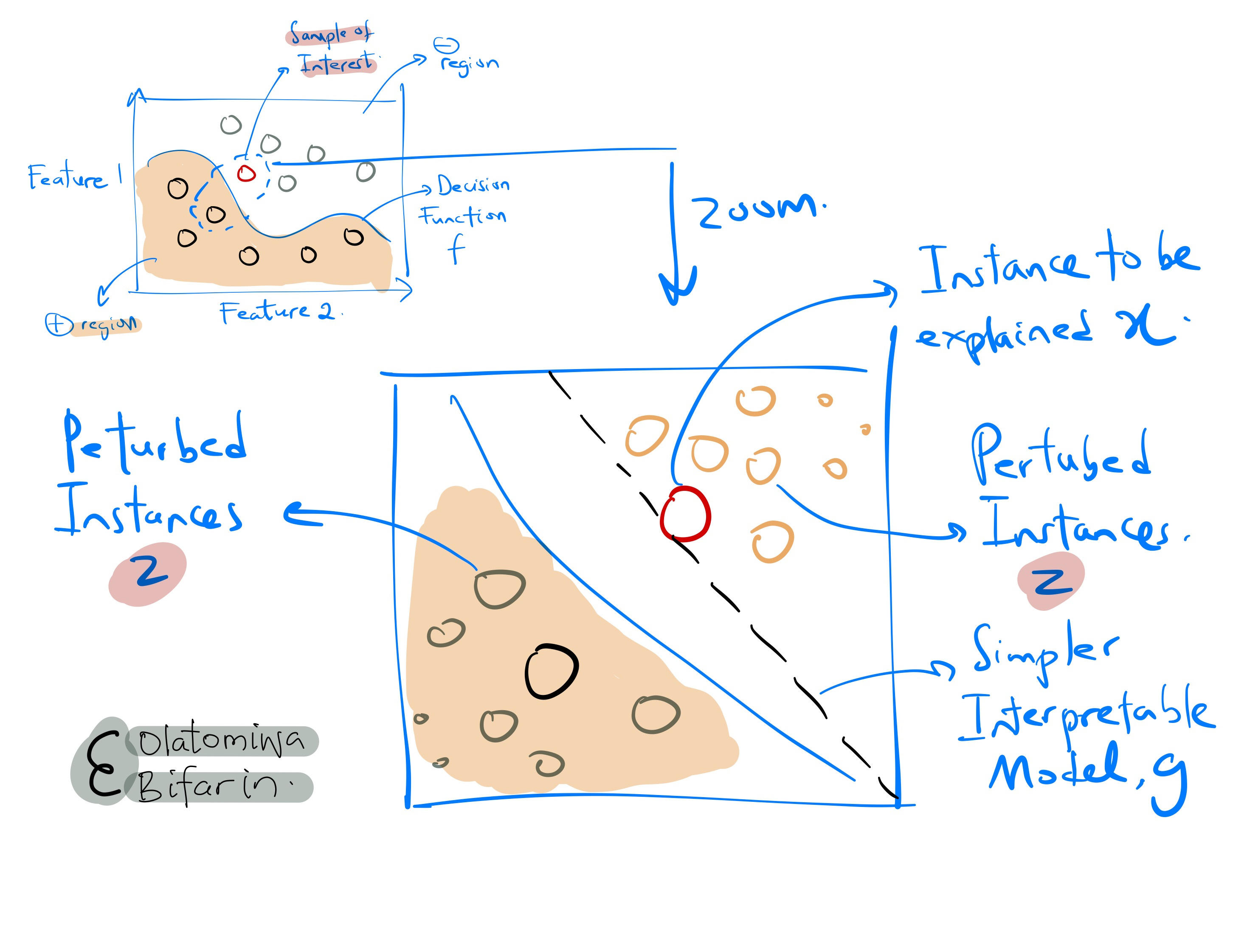
LIME explains the prediction of an individual instance by approximating the model with a simpler interpretable model, such as a linear model or a decision tree. This approximation is made by creating perturbed versions of the original instance in the “neighborhood” of the instance and training an interpretable model on those perturbed instances (We will get into what all these mean in a second).
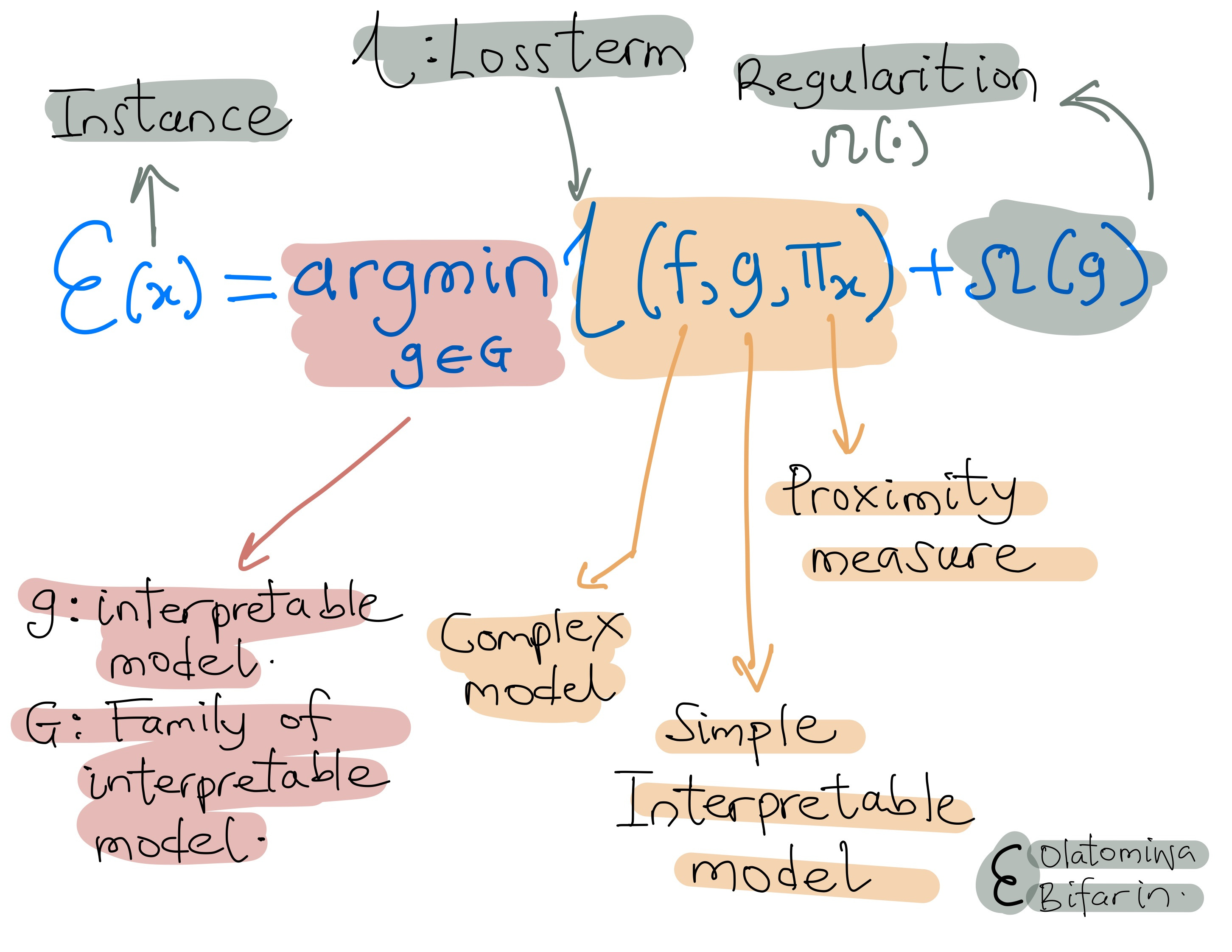
In the meantime, let us represent LIME formally with the equation below:
Next, let’s see how the algorithm works:
Sample of Interest
Here I show a sample of interest to be explained, and the decision boundary of the original model used to fit the data.
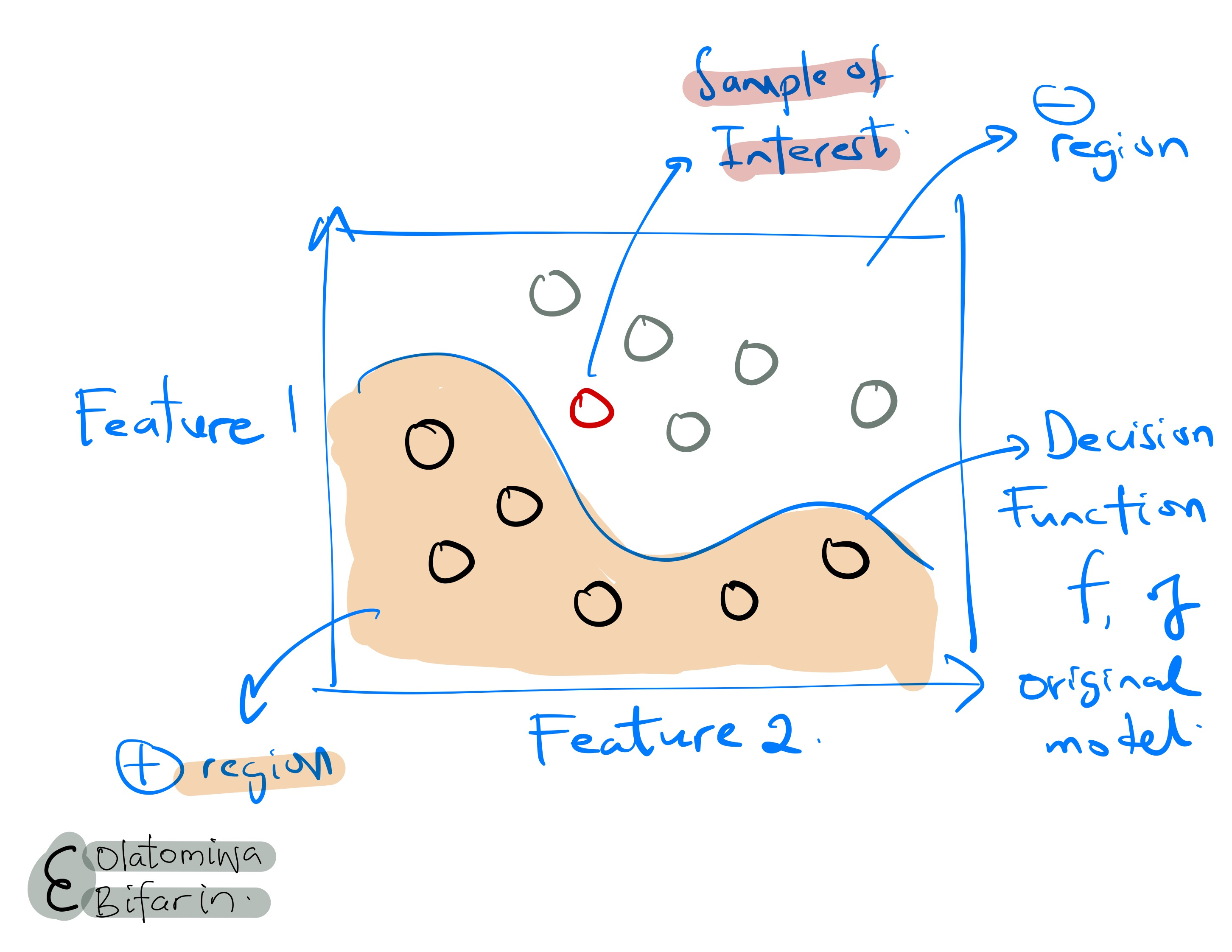
Sampling
Given an instance to be explained, LIME sample instances in its vicinity. The samples are generated by perturbing the original instance by adding noise and keeping only the instances close to the original instance.
Weighting
LIME assigns each synthetic instance (from the step above) a weight based on its proximity to the original instance. The weights reflect how much each synthetic instance influences the prediction for the instance being explained.
Fitting
LIME fits an interpretable model, such as a linear regression model (or a decision tree), to the weighted samples generated in step above. The interpretable model approximates the behavior of the complex model locally, around the instance to be explained.
The locally aware loss function (loss term from equation 1 above ) is illustrated below:
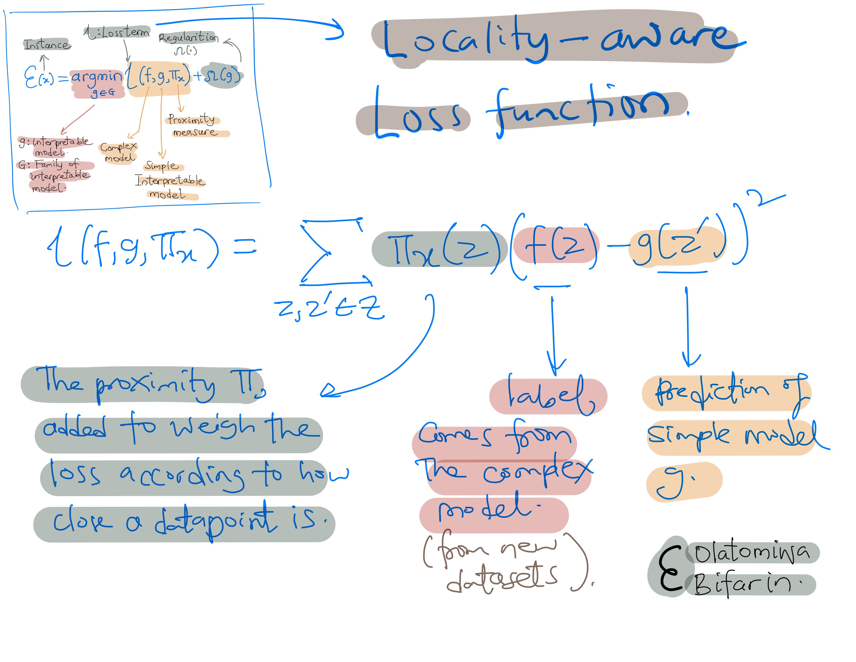
LIME's objective is to discover an explanation model, labeled as g, which minimizes the locality-aware loss L(f, g, Πx). Here, f denotes the black box model requiring explanation, and Πx represents the proximity measure.
In brief, the locality-aware loss quantifies the difference between the explanation model and the original model within the specified locality.
Explanation
LIME then presents the influential features and their contributions from the interpretable model g visually, in a human-understandable format, such as a bar chart or a table.
Let’s illustrate with the iris dataset. It contains measurements of 150 iris flowers from three different species: setosa, versicolor, and virginica. For each flower, the dataset includes four features: the lengths and the widths of the sepals and petals.

The task we're addressing here is a multiclass classification problem. The goal is to train a model that can accurately predict the species of an iris flower based on the four features provided.
In the code below, I trained a Random Forest Classifier followed by using LIME to explain the prediction of one of the instances.
from sklearn.datasets import load_iris
from sklearn.model_selection import train_test_split

# Load and process data
iris = load_iris()
X_train, X_test, y_train, y_test = train_test_split(iris.data, iris.target, random_state=42)
from sklearn.ensemble import RandomForestClassifier

# Classifier
rf = RandomForestClassifier(random_state=42)
rf.fit(X_train, y_train)
from sklearn.metrics import accuracy_score

predictions = rf.predict(X_test)
print("Accuracy: ", accuracy_score(y_test, predictions))

# Explanation with LIME
from lime.lime_tabular import LimeTabularExplainer

explainer = LimeTabularExplainer(X_train, feature_names=iris.feature_names, class_names=iris.target_names, discretize_continuous=True)

i = 1  # instance to be explained
exp = explainer.explain_instance(X_test[i], rf.predict_proba, num_features=4, top_labels=1)

# Generate the plot for the top label
fig = exp.as_pyplot_figure(label=0)

The graph above shows an explanation for a correct prediction for Setosa.
In brief, the bar graph shows the values of the LIME coefficients for each feature. The higher the (absolute) value of the coefficient, the more important the feature is for the model's prediction.
In this case, the most important feature is the petal width, followed by the petal length. Furthermore, the petal width, sepal width, and the sepal length drive the prediction towards Setosa, while the petal length drives the prediction towards ‘NOT setosa’
In summary, LIME approximates the behavior of the complex model locally by a simple interpretable model and provides the explanation in a human-understandable format.